We have learned about individual neurons in the previous section, now it’s time to put them together to form an actual neural network.
The idea is quite simple – we line multiple neurons up to form a layer, and connect the output of the first layer to the input of the next layer. Here is an illustration:
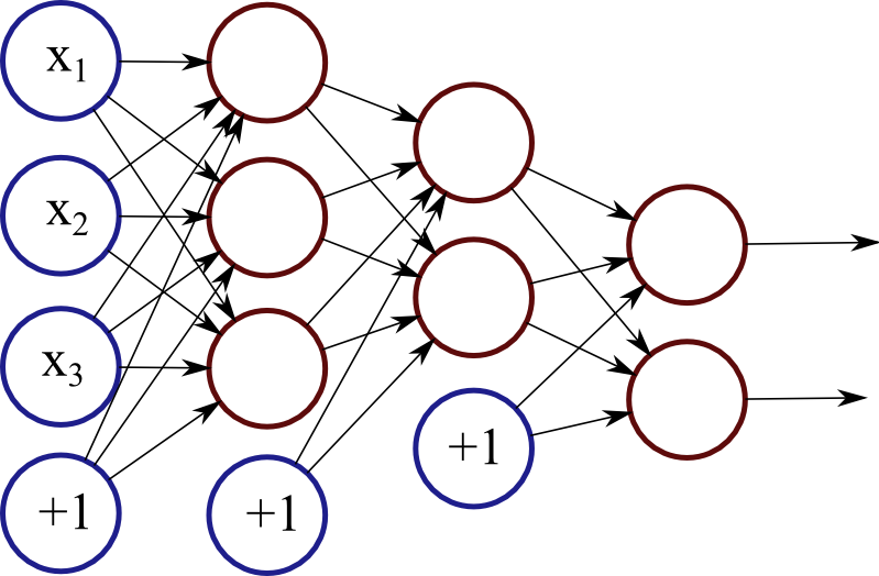
Each red circle in the diagram represents a neuron, and the blue circles represent fixed values. From left to right, there are four columns: the input layer, two hidden layers, and an output layer. The output from neurons in the previous layer is directed into the input of each of the neurons in the next layer.
We have 3 features (vector space dimensions) in the input layer that we use for learning: \(x_1\), \(x_2\) and \(x_3\). The first hidden layer has 3 neurons, the second one has 2 neurons, and the output layer has 2 output values. The size of these layers is up to you – on complex real-world problems we would use hundreds or thousands of neurons in each layer.
The number of neurons in the output layer depends on the task. For example, if we have a binary classification task (something is true or false), we would only have one neuron. But if we have a large number of possible classes to choose from, our network can have a separate output neuron for each class.
The network in Figure 1 is a deep neural network, meaning that it has two or more hidden layers, allowing the network to learn more complicated patterns. Each neuron in the first hidden layer receives the input signals and learns some pattern or regularity. The second hidden layer, in turn, receives input from these patterns from the first layer, allowing it to learn “patterns of patterns” and higher-level regularities. However, the cost of adding more layers is increased complexity and possibly lower generalisation capability, so finding the right network structure is important.
Implementation
I have implemented a very simple neural network for demonstration. You can find the code here: SimpleNeuralNetwork.java
The first important method is initialiseNetwork(), which sets up the necessary structures:
	public void initialiseNetwork(){
		input = new double[1 + M]; // 1 is for the bias
		hidden = new double[1 + H];
		weights1 = new double[1 + M][H];
		weights2 = new double[1 + H];

		input[0] = 1.0; // Setting the bias
		hidden[0] = 1.0;
	}
\(M\) is the number of features in the feature vectors, \(H\) is the number of neurons in the hidden layer. We add 1 to these, since we also use the bias constants.
We represent the input and hidden layer as arrays of doubles. For example, hidden[i] stores the current output value of the i-th neuron in the hidden layer.
The first set of weights, between the input and hidden layer, are stored as a matrix. Each of the \((1 + M)\) neurons in the input layer connects to \(H\) neurons in the hidden layer, leading to a total of \((1 + M) \times H\) weights. We only have one output neuron, so the second set of weights between hidden and output layers is technically a \((1 + H) \times 1\) matrix, but we can just represent that as a vector.
The second important function is forwardPass(), which takes an input vector and performs the computation to reach an output value.
	public void forwardPass(){
		for(int j = 1; j < hidden.length; j++){
			hidden[j] = 0.0;
			for(int i = 0; i < input.length; i++){
				hidden[j] += input[i] * weights1[i][j-1];
			}
			hidden[j] = sigmoid(hidden[j]);
		}

		output = 0.0;
		for(int i = 0; i < hidden.length; i++){
			output += hidden[i] * weights2[i];
		}
		output = sigmoid(output);
	}
The first for-loop calculates the values in the hidden layer, by multiplying the input vector with the weight vector and applying the sigmoid function. The last part calculates the output value by multiplying the hidden values with the second set of weights, and also applying the sigmoid.
Evaluation
To test out this network, I have created a sample dataset using the database at quandl.com. This dataset contains sociodemographic statistics for 141 countries:
- Population density (per suqare km)
- Population growth rate (%)
- Urban population (%)
- Life expectancy at birth (years)
- Fertility rate (births per woman)
- Infant mortality (deaths per 1000 births)
- Enrolment in tertiary education (%)
- Unemployment (%)
- Estimated control of corruption (score)
- Estimated government effectiveness (score)
- Internet users (per 100)
Based on this information, we want to train a neural network that can predict whether the GDP per capita is more than average for that country (label 1 if it is, 0 if it’s not).
I’ve separated the dataset for training (121 countries) and testing (40 countries). The values have been normalised, by subtracting the mean and dividing by the standard deviation, using a script from a previous article. I’ve also pre-trained a model that we can load into this network and evaluate. You can download these from here: original data, training data, test data, pretrained model.
You can then execute the neural network (remember to compile and link the binaries):
java neuralnet.SimpleNeuralNetwork data/model.txt data/countries-classify-gdp-normalised.test.txt
The output should be something like this:
Label: 0	Prediction: 0.01
Label: 0	Prediction: 0.00
Label: 1	Prediction: 0.99
Label: 0	Prediction: 0.00
...
Label: 0	Prediction: 0.20
Label: 0	Prediction: 0.01
Label: 1	Prediction: 0.99
Label: 0	Prediction: 0.00
Accuracy: 0.9
The network is in verbose mode, so it prints out the labels and predictions for each test item. At the end, it also prints out the overall accuracy. The test data contains 14 positive and 26 negative examples; a random system would have had accuracy 50%, whereas a biased system would have accuracy 65%. Our network managed 90%, which means it has learned some useful patterns in the data.
In this case we simply loaded a pre-trained model. In the next section, I will describe how to learn this model from some training data.
Pingback:Neural Networks, Part 2: The Neuron | Marek ReiMarek Rei