Menu Close

Author: Marek

Analysing NLP publication patterns

Recently, I got curious about finding out how much different institutions publish in my area. Does Google publish more than Microsoft? Which university has the strongest publication record in NLP? And are there any interesting trends that can be seen in the recent years? Quantity does not necessarily equal quality, but the number of publications is still a reasonable indicator of general activity in the field, how big the research group is, and how outward-facing are the research projects.

My approach was to crawl papers from the 6 biggest conferences that are relevant to my research: ACL, EACL, NAACL, EMNLP, NIPS, ICML. The first 4 focus on NLP applications regardless of methods, and the latter 2 on machine learning algorithms regardless of tasks. The time window was restricted to 2012-2016, as I’m more interested in current publications.

Luckily, all these conferences have nice webpages listing all the papers published there. ACL Anthology contains records for ACL, EACL, NAACL and EMNLP, NIPS has a separate webpage for papers, and ICML proceedings are on the JMLR website (except for ICML12 which are on the conference website). I wrote python scripts that crawled all the papers from these conferences, extracting author names and organisations. While authors can be crawled directly from the websites, in order to find the organisation names I had to parse the pdfs into text and extract anything that looked like a university or company name in the first 30 lines of on the paper. I wrote a bunch of manual patterns to map names to canonical versions (“UCL” to “University College London” and “Google Inc” to “Google”), although it is likely that I still missed some edge cases.

Theano Tutorial

This is an introductory tutorial on using Theano, the Python library. I’m going to start from scratch and assume no previous knowledge of Theano. However, understanding how neural networks work will be useful when getting to the code examples towards the end.

The plan for the tutorial is as follows:

  1. Give a basic introduction to Theano and explain the important concepts.
  2. Go over the main operations that we have available in Theano.
  3. Look at working code examples.

I recently gave this tutorial as a talk in University of Cambridge and it turned out to be way more popular than expected. In order to give more people access to the material, I’m now writing it up as a blog post.

I do not claim to know everything about Theano, and I constantly learn new things myself. If you find any errors or have suggestions on how to improve this tutorial, do let me know.

The code examples can be found in the Github repository: https://github.com/marekrei/theano-tutorial

1. What is Theano?

CYh2GMnWkAELDTL

Theano is a Python library for efficiently handling mathematical expressions involving multi-dimensional arrays (also known as tensors). It is a common choice for implementing neural network models. Theano has been developed in University of Montreal, in a group led by Yoshua Bengio, since 2008.

Some of the features include:

  • automatic differentiation – you only have to implement the forward (prediction) part of the model, and Theano will automatically figure out how to calculate the gradients at various points, allowing you to perform gradient descent for model training.
  • transparent use of a GPU – you can write the same code and run it either on CPU or GPU. More specifically, Theano will figure out which parts of the computation should be moved to the GPU.
  • speed and stability optimisations – Theano will internally reorganise and optimise your computations, in order to make them run faster and be more numerically stable. It will also try to compile some operations into C code, in order to speed up the computation.

Online Representation Learning in Recurrent Neural Language Models

In a basic neural language model, we optimise a fixed set of parameters based on a training corpus, and predictions on an unseen test set are a direct function of these parameters. What if instead of a static model we constantly measured the types of errors the model is making and adjust the parameters accordingly? It would potentially be more closer to how humans operate, constantly making small adjustments in their decisions based on feedback.

The necessary information is already available – language models use the previous word in the sequence as context, which means they know the correct answer for the previous time step (or at least need to assume they know). We can use this to calculate error derivatives at each time step and update parameters even during testing. This sounds like it would require loads of extra computation at test time, but by updating only a small part of the model we can actually get better results with faster execution and fewer parameter.

This post is a summary of my EMNLP 2015 paper “Online Representation Learning in Recurrent Neural Language Models“.

RNNLM

First a short description of the RNN language model that I use as a baseline. It follows the implementation by Mikolov et al. (2011) in the RNNLM Toolkit.

rnnlm

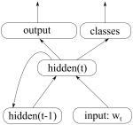
The previous word goes into the network as a 1-hot vector which is then multiplied with a weight matrix, giving us a corresponding word embedding. This, together with the previous hidden state, act as input to the current hidden state of the network:

\(hidden_t = \sigma(E \cdot input_t + W_h \cdot hidden_{t-1})\)

26 Things I Learned in the Deep Learning Summer School

In the beginning of August I got the chance to attend the Deep Learning Summer School in Montreal. It consisted of 10 days of talks from some of the most well-known neural network researchers. During this time I learned a lot, way more than I could ever fit into a blog post. Instead of trying to pass on 60 hours worth of neural network knowledge, I have made a list of small interesting nuggets of information that I was able to summarise in a paragraph.

At the moment of writing, the summer school website is still online, along with all the presentation slides. All of the information and most of the illustrations come from these slides and are the work of their original authors. The talks in the summer school were filmed as well, hopefully they will also find their way to the web.

Update: the Deep Learning Summer School videos are now online.

Alright, let’s get started.

1. The need for distributed representations

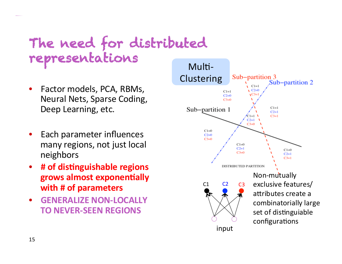
During his first talk, Yoshua Bengio said “This is my most important slide”. You can see that slide below:dlss-3aug2015

Let’s say you have a classifier that needs to detect people that are male/female, have glasses or don’t have glasses, and are tall/short. With non-distributed representations, you are dealing with 2*2*2=8 different classes of people. In order to train an accurate classifier, you need to have enough training data for each of these 8 classes. However, with distributed representations, each of these properties could be captured by a different dimension. This means that even if your classifier has never encountered tall men with glasses, it would be able to detect them, because it has learned to detect gender, glasses and height independently from all the other examples.

Transforming Images to Feature Vectors

I’m keen to explore some challenges in multimodal learning, such as jointly learning visual and textual semantics. However, I would rather not start by attempting to train an image recognition system from scratch, and prefer to leave this part to researchers who are more experienced in vision and image analysis.

Therefore, the goal is to use an existing image recognition system, in order to extract useful features for a dataset of images, which can then be used as input to a separate machine learning system or neural network. We start with a directory of images, and create a text file containing feature vectors for each image.

1. Install Caffe

Caffe is an open-source neural network library developed in Berkeley, with a focus on image recognition. It can be used to construct and train your own network, or load one of the pretrained models. A web demo is available if you want to test it out.

Follow the installation instructions to compile Caffe. You will need to install quite a few dependencies (Boost, OpenCV, ATLAS, etc), but at least for Ubuntu 14.04 they were all available in public repositories.

Once you’re done, run

make test
make runtest

This will run the tests and make sure the installation is working properly.

Linguistic Regularities in Word Representations

In 2013, Mikolov et al. (2013) published a paper showing that complicated semantic analogy problems could be solved simply by adding and subtracting vectors learned with a neural network. Since then, there has been some more investigation into what is actually behind this method, and also some suggested improvements. This post is a summary/discussion of the paper “Linguistic Regularities in Sparse and Explicit Word Representations“, by Omer Levy and Yoav Goldberg, published at ACL 2014.

The Task

The task under consideration is analogy recovery. These are questions in the form:

a is to b as c is to d

In a usual setting, the system is given words a, b, c, and it needs to find d. For example:

‘apple’ is to ‘apples’ as ‘car’ is to ?

where the correct answer is ‘cars’. Or the well-known example:

‘man’ is to ‘woman’ as ‘king’ is to ?

where the desired answer is ‘queen’.

While methods such as relation extraction would also be completely reasonable approaches to this problem, the research is mainly focused on solving it by using vector similarity methods. This means we create vector representations for each of the words, and then use their positions in the high-dimensional feature space to determine what the missing word should be.

Multilingual Semantic Models

In this post I’ll discuss a model for learning word embeddings, such that they end up in the same space in different languages. This means we can find the similarity between some English and German words, or even compare the meaning of two sentences in different languages. It is a summary and analysis of the paper by Karl Moritz Hermann and Phil Blunsom, titled “Multilingual Models for Compositional Distributional Semantics“, published at ACL 2014.

The Task

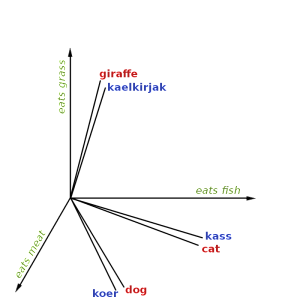
The goal of this work is to extend the distributional hypothesis to multilingual data and joint-space embeddings. This would give us the ability to compare words and sentences in different languages, and also make use of labelled training data from languages other than the target language. For example, below is an illustration of English words and their Estonian translations in the same semantic space.

vector_space_model_multilingual


This actually turns out to be a very difficult task, because the distributional hypothesis stops working across different languages. While “fish” is an important feature of “cat”, because they occur together often, “kass” never occurs with “fish”, because they are in different languages and therefore used in separate sets of documents.

In order to learn these representations in the same space, the authors construct a neural network that learns from parallel sentences (pairs of the same sentence in different languages). The model is then evaluated on the task of topic classification, training on one language and testing on the other.

Political ideology detection

Neural networks have a range of interesting applications, and here I will discuss on one them: recursive neural networks and the detection of political ideology. This post is a summary and analysis of a recent publication by Mohit Iyyer, Peter Anns, Jordan Boyd-Graber and Philip Resnik: “Political Ideology Detection Using Recursive Neural Networks“.

The Task

Given a sentence, we want the model to detect the political ideology expressed in that sentence. In this research, the authors deal with US politics, so the possible options are liberal (democrats) or conservative (republicans). As a practical application we might consider a system that processes a large amount of news articles or public speeches to detect and measure explicit or hidden political bias of the authors.

democrat-republican

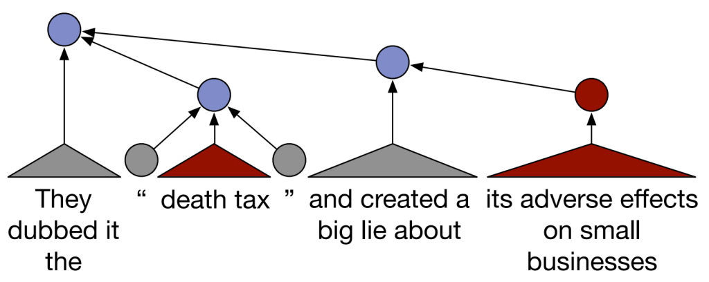
A traditional approach to this problem is a simple bag-of-words model, where each word is treated as a separate feature, but this ignores any syntactic structure and even word order. As shown below, political ideology can be compositionally complicated – while certain sections of the sentence are locally conservative, the way they are used in context makes the overall sentence liberal.political_sample_1

Figure 1: Sample sentence from Iyyer et al. (2014). Blue nodes are liberal, red nodes are conservative, grey nodes are neutral.

Don’t count, predict

In the past couple of years, neural networks have nearly taken over the field of NLP, as they are being used in recent state-of-the-art systems for many tasks. One interesting application is distributional semantics, as they can be used to learn intelligent dense vector representations for words. Marco Baroni, Georgiana Dinu and German Kruszewski presented a paper in ACL 2014 called “Don’t count, predict! A systematic comparison of context-counting vs. context-predicting semantic vectors“, where they compare these new neural-network models with more traditional context vectors on a range of different tasks. Here I will try to give an overview and a summary of their work.

Distributional hypothesis

The goal is to find how similar two words are to each other semantically. The distributional hypothesis states:

Words which are similar in meaning occur in similar contexts
(Rubenstein & Goodenough, 1965).

Therefore, if we want to find a word similar to “magazine”, we can look for words that occur in similar contexts, such as “newspaper”.

I was reading a magazine today I was reading a newspaper today
The magazine published an article The newspaper published an article
He buys this magazine every day He buys this newspaper every day


Also, if we want to find how similar “magazine” and “newspaper” are, we can compare how similar are all the contexts in which they appear. For example, to find the similarity between two words, we can represent the contexts as feature vectors and calculate the cosine similarity between their corresponding vectors.

Neural Networks, Part 3: The Network

We have learned about individual neurons in the previous section, now it’s time to put them together to form an actual neural network.

The idea is quite simple – we line multiple neurons up to form a layer, and connect the output of the first layer to the input of the next layer. Here is an illustration:

neuralnetwork
Figure 1: Neural network with two hidden layers.

Each red circle in the diagram represents a neuron, and  the blue circles represent fixed values. From left to right, there are four columns: the input layer, two hidden layers, and an output layer. The output from neurons in the previous layer is directed into the input of each of the neurons in the next layer.

We have 3 features (vector space dimensions) in the input layer that we use for learning: \(x_1\), \(x_2\) and \(x_3\). The first hidden layer has 3 neurons, the second one has 2 neurons, and the output layer has 2 output values. The size of these layers is up to you – on complex real-world problems we would use hundreds or thousands of neurons in each layer.