Online Representation Learning in Recurrent Neural Language Models

In a basic neural language model, we optimise a fixed set of parameters based on a training corpus, and predictions on an unseen test set are a direct function of these parameters. What if instead of a static model we constantly measured the types of errors the model is making and adjust the parameters accordingly? It would potentially be more closer to how humans operate, constantly making small adjustments in their decisions based on feedback.

The necessary information is already available – language models use the previous word in the sequence as context, which means they know the correct answer for the previous time step (or at least need to assume they know). We can use this to calculate error derivatives at each time step and update parameters even during testing. This sounds like it would require loads of extra computation at test time, but by updating only a small part of the model we can actually get better results with faster execution and fewer parameter.

This post is a summary of my EMNLP 2015 paper “Online Representation Learning in Recurrent Neural Language Models“.

RNNLM

First a short description of the RNN language model that I use as a baseline. It follows the implementation by Mikolov et al. (2011) in the RNNLM Toolkit.

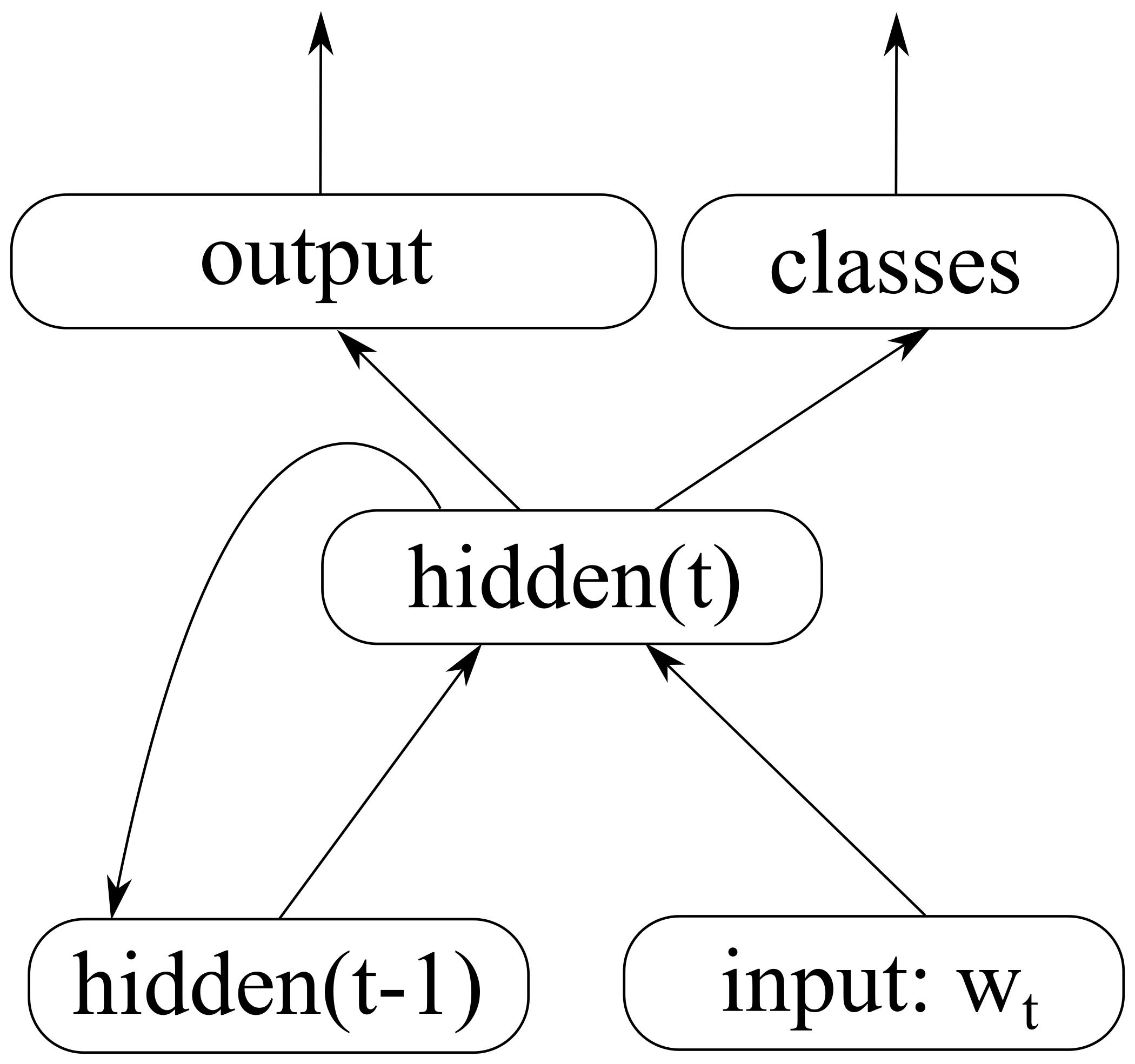
The previous word goes into the network as a 1-hot vector which is then multiplied with a weight matrix, giving us a corresponding word embedding. This, together with the previous hidden state, act as input to the current hidden state of the network:

\(hidden_t = \sigma(E \cdot input_t + W_h \cdot hidden_{t-1})\)

The hidden state is connected to the output layer, which predicts the next word in the sequence. In order to avoid performing a softmax operation over the whole vocabulary, all words are divided between classes and the probability of the next word is factored into the probability of the class and the probability of the next word given the class:

\(P(w_{t+1} | w_{1}^{t}) \approx classes_c \cdot output_{w_{t+1}}\)

\(classes = softmax(W_c \cdot hidden_t)\)

\(output = softmax(W_o^{(c)} \cdot hidden_t)\)

The words are divided into classes by frequency-based bucketing (following Mikolov et al., 2011), and the learning rate is divided by 2 if the improvement is not sufficient. The RNNLM Toolkit treats the training data as a continuous stream of tokens and performs backpropagation through time for a fixed number of steps – the text is essentially split into fixed-sized chunks for optimisation. Instead, we perform sentence splitting and backpropagate errors from the end of each sentence to the beginning.

RNNLM with online learning

Let’s introduce a special vector into the model, which will represent the current unit of text being processed (a sentence, a paragraph, or a document). We can then update it after each prediction, based on the errors the model has made on that document.

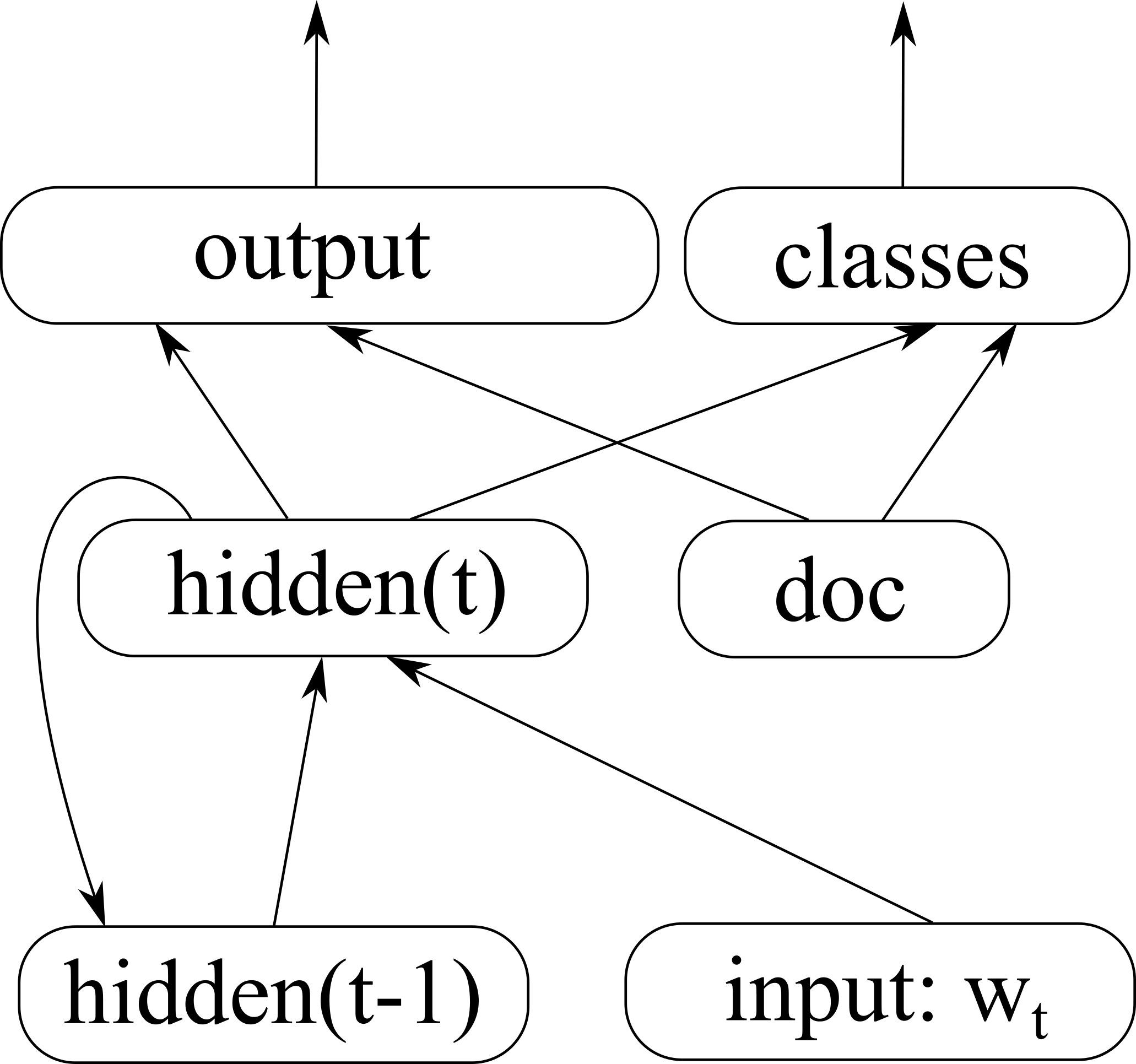
The output probabilities over classes and words are then conditioned on this new document vector:

\(classes = softmax(W_c \cdot hidden_t + W_{dc} \cdot doc)\)
\(output = softmax(W_o^{(c)} \cdot hidden_t + W_{do}^{(c)} \cdot doc)\)

Notice that there is no input going into the document vector. Instead of constructing it iteratively, like the values in a hidden layer, we treat it as a vector of parameters and optimise them both during training and testing. After predicting each word, we calculate the error in the output layer, backpropagate this into the document vector, and adjust the values. While the main language model is a smoothed static representation of the training data, the document vector will contain information about how a specific sentence/document differs from this main language model.

The document vector is connected directly to the output layers of the RNNLM, in parallel to the hidden layer. This allows us to update the document vector after every step, instead of waiting until the end of the sentence to perform backpropagation through time.

Le and Mikolov (2014) used a related approach for learning vector representations of sentences and achieved good results on the sentiment detection task. They added a vector for a sentence into a feedforward language model, stepped through the sentence, and used the values at the last step as a representation of that sentence. While they connected the vector as part of the input layer, we have connected it directly to the output layer – in an RNNLM the input layer only gets updated at the end of the sentence (during backpropagation-through-time), whereas we want to update the document vector after each time step.

Experiments

We constructed a dataset from English Wikipedia to evaluate language modelling performance of the two models. The text was tokenised, sentence split and lowercased. The sentences were shuffled, in order to minimise any transfer effects between consecutive sentences, and then split into training, development and test sets. The final sentences were sampled randomly, in order to obtain reasonable training times for the experiments. Dataset sizes are as follows:

[table]
, Train, Dev, Test
Words, 9\,990\,782, 237\,037, 4\,208\,847
Sentences, 419\,278, 10\,000, 176\,564
[/table]

The regular RNNLM with a 100-dimensional hidden layer (M = 100) and no document vector (D=0) is the baseline. In the experiments we increase the capacity of the model using different methods and measure how that affects the perplexity on the datasets.

[table]
, Train PPL , Dev PPL , Test PPL
Baseline M=100 , 92.65 , 103.56 , 102.51
M=120 , 88.60 , 98.78 , 97.79
M=100\, D=20 , 87.28 , 95.36 , 94.39
M=135 , 85.17 , 96.33 , 95.71
M=100\, D=35 , 80.11 , 91.05 , 90.29
[/table]

Increasing the hidden layer size M does improve the model performance and perplexity decreases from 102.51 to 95.71. However, adding the same number of neurons into the actively-updated document vector gives an even lower perplexity of 90.29.

 Experiments with semantic similarity

The resulting document vector can also be used for calculating semantic similarity between texts. We sampled random sentences from the development data, processed them with the language model, and used the resulting document vector to find 3 most similar sentences in the development set. Below are some examples.

Input: Both Hufnagel and Marston also joined the long-standing technical death metal band Gorguts.

• The band eventually went on to become the post-hardcore band Adair.
• The band members originally came from different death metal bands, bonding over a common interest in d-beat.
• The proceeds went towards a home studio, which enabled him to concentrate on his solo output and songs that were to become his debut mini-album “Feeding The Wolves”.

Input: The Chiefs reclaimed the title on September 29, 2014 in a Monday Night Football game against the New England Patriots, hitting 142.2 decibels.

• He played in twenty-four regular season games for the Colts, all off the bench.
• In May 2009 the Warriors announced they had re-signed him until the end of the 2011 season.
• The team played inconsistently throughout the campaign from the outset, losing the opening two matches before winning four consecutive games during September 1927.

Input: He was educated at Llandovery College and Jesus College, Oxford, where he obtained an M.A. degree.

• He studied at the Orthodox High School, then at the Faculty of Mathematics.
• Kaigama studied for the priesthood at St. Augustine’s Seminary in Jos with further study in theology in Rome.
• Under his stewardship, Zahira College became one of the leading schools in the country.

Summary

There has been a lot of work on developing static models for machine learning – we train the model parameters on the training data and then apply them on the test data. However, there is a lot of potential for dynamical models, which take advantage of immediate feedback signals and are able to continuously adjust the model parameters. Our experiment showed that, at least for language modelling, such a model is indeed a viable option.