In this post I’ll discuss a model for learning word embeddings, such that they end up in the same space in different languages. This means we can find the similarity between some English and German words, or even compare the meaning of two sentences in different languages. It is a summary and analysis of the paper by Karl Moritz Hermann and Phil Blunsom, titled “Multilingual Models for Compositional Distributional Semantics“, published at ACL 2014.
The Task
The goal of this work is to extend the distributional hypothesis to multilingual data and joint-space embeddings. This would give us the ability to compare words and sentences in different languages, and also make use of labelled training data from languages other than the target language. For example, below is an illustration of English words and their Estonian translations in the same semantic space.
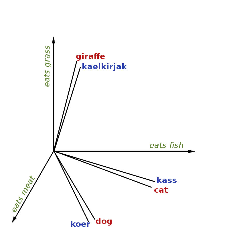
This actually turns out to be a very difficult task, because the distributional hypothesis stops working across different languages. While “fish” is an important feature of “cat”, because they occur together often, “kass” never occurs with “fish”, because they are in different languages and therefore used in separate sets of documents.
In order to learn these representations in the same space, the authors construct a neural network that learns from parallel sentences (pairs of the same sentence in different languages). The model is then evaluated on the task of topic classification, training on one language and testing on the other.
A bit of a spoiler, but here is a visualisation of some words from the final model, mapped into 2 dimensions.
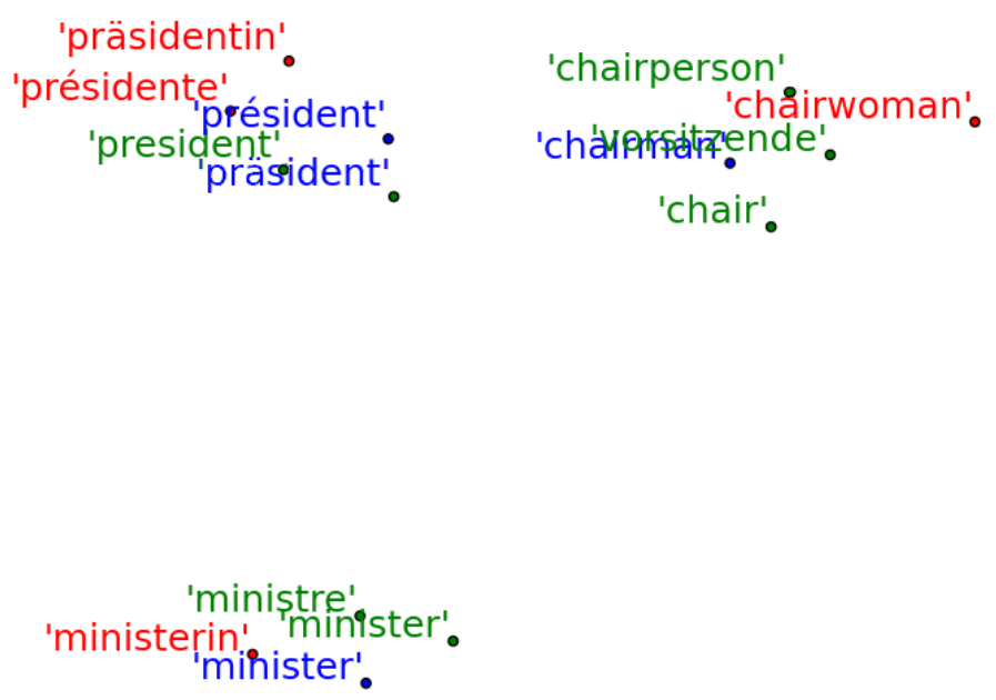
The words from English, German and French are successfully mapped into clusters based on meaning. The colours indicate gender (blue=male, red=female, green=neutral).
The Multilingual Model
The main idea is as follows: We have sentence \(a\) in one language, and we have a function \(f(a)\) which maps that sentence into a vector representation (we’ll come back to that function). We then have sentence \(b\), which is the same sentence just in a different language, and function \(g(b)\) for mapping it into a vector representation. Our goal is to have \(f(a)\) and \(g(b)\) be identical, because both of these sentences have the same meaning. So during training, we show the model a series of parallel sentences \(a\) and \(b\), and each time we adjust the functions \(f(a)\) and \(g(b)\) so that they would produce more similar vectors.
Here is a graphical representation of the model:
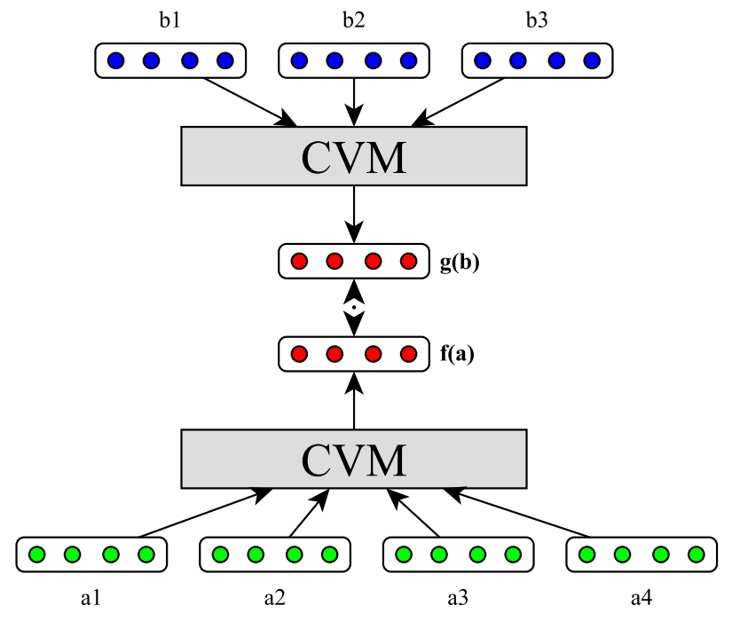
\(b1\), \(b2\) and \(b3\) are words in sentence \(b\); \(a1\), \(a2\),\(a3\) and \(a4\) are words in sentence \(a\). The red vectors in the middle are the sentence representations that we want to be similar.
Next, let’s talk about the functions \(f(a)\) and \(g(b)\) that map a sentence to a vector. As you can see from the image above, each word is represented as a vector as well. The simplest option of going from words to sentences is to just add the individual word vectors together (the ADD model):
\(f_{ADD}(a) = \sum_{i=1}^{n} a_i\)
Here, \(a_i\) is the vector for word number \(i\) in sentence \(a\). This addition is similar to a basic bag-of-words model, because it doesn’t preserve any information about the order of the words. Therefore, the authors have also proposed a bigram version of this function (the BI model):
\(f_{BI}(a) = \sum_{i=1}^{n} tanh(a_{i-1} + a_i)\)
In this function, we step though the sentence, add together vectors for two consecutive words, and pass them through a nonlinearity (tanh). The result is then summed together into a sentence vector. This is essentially a multi-layer compositional network, where word vectors are first combined to bigram vectors, and then bigram vectors are combined to sentence vectors.
One more component to make this model work – the optimization function. The authors define an energy function given two sentences:
\(E(a,b) = || f(a) – g(b) ||^ 2\)
This means we find the Euclidean distance between the two vector representations and take the square of it. This value will be big when the vectors are different, and small when they are similar.
But we can’t directly use this for optimization, because functions \(f(a)\) and \(g(b)\) that always returned zero vectors would be the most optimal solution. We want the model to give similar vectors for similar sentences, but different vectors for semantically different sentences. Here’s a function for that:
\(E_{nc}(a,b,c) = [m + E(a,b) – E(a,c)]_{+}\)
We’ve introduced a randomly selected sentence \(c\) that probably has nothing to do with \(a\) or \(b\). Our objective is to minimze the \(E_{nc}(a,b,c)\) function, which means we want \(E(a,b)\) (for related sentences) to be small, and \(E(a,c)\) (for unrelated sentences) to be large. This form of training – teaching the model to distinguish between correct and incorrect samples – is called noise contrastive estimation. The formula also includes \(m\), which is the margin we want to have between the values of \(E(a,b)\) and \(E(a,c)\). The whole thing is passed through the function \([x]_{+} = max(x,0)\), which means that if \(E(a,c)\) is greater than \(E(a,b)\) by margin \(m\), then we’re already optimal and don’t need to adjust the model further.
The authors also experiment with a document-level variation of the model (the DOC model), where individual sentence vectors are combined into document vectors and these are also optimized to be similar, in addition to the sentence vectors.
Evaluation
The authors evaluate the system on the task of topic classification. The classifier is trained on one language (eg English) and the test results are reported on another language (eg German) for which no labelled training data was used. They run two main experiments:
- The cross-lingual document classification (CLDC) task, described by Klementiev et al. (2012). The system is trained on the parallel Europarl corpus, and tested on Reuters RCV1/RCV2. The language pairs used were English-German and English-French.
- The authors built a new corpus from parallel subtitles of TED talks (not yet online at the time of writing this), based on a previous TED corpus for IWSLT. Each talk also has topic tags assigned to them, and the task is to assign a correct tag to every talk, using the document-level vector.
Results
First, results on the CLDC task:
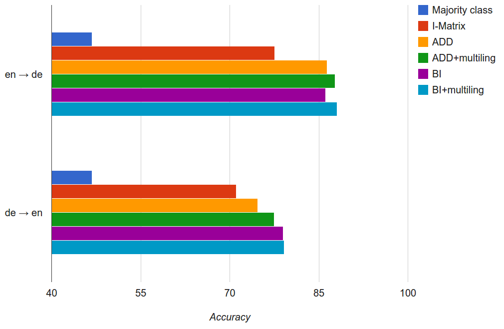
I-Matrix is the previous state-of-the-art system, and all the models described here manage to outperform it. The +-variations of the model (ADD+ and BI+) use the French data as an extra training resource, thereby improving performance. This is an interesting result, as the classifier is trained on English and tested on German, and French seems completely unrelated to the task. But by adding it into the model, the English word representations are improved by having more information available, which in turn propagates on to having better German representations.
Next, experiments on the TED corpus:
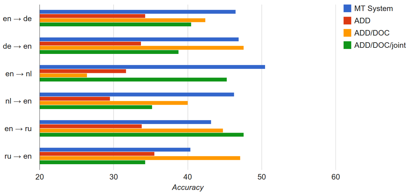
The authors have performed a much larger number of experiments, and I’ve only chosen a few examples to show here.
The MT System is a machine translation baseline, where the test data is translated into the source language using a machine translation system. The most interesting scenarios for application are where the source language is English, and this is where the MT baseline often still wins. So if we want to topic classification in Dutch, but we only have English labelled data, it’s best to just automatically translate the Dutch text into English before classification.
Experiments in the other direction (where the target language is English) show different results, and the multilingual neural models manage to win on most languages. I’m curious about this difference – perhaps the MT systems are better tuned to translate into English, but not as good when translating from English into other languages? In any case, I think with some additional developments the neural network model will be able to beat the baseline in both directions.
In most cases, adding the document-level training signal (ADD/DOC) helped accuracy quite a bit. The bigram models (BI) however were outperformed by the basic ADD models on this task, and the authors suspect this is due to sparsity issues caused by less training data.
Finally, the ADD/DOC/joint model was trained on all languages simultaneously, taking advantage of parallel data in all the languages, and mapping all vectors into the same space. The results of this experiment seem to be mixed, leading to an improvement on some languages and decrease on others.
In conclusion, this is definitely a very interesting model, and it bridges the gap between vector representations of different languages, using only sentence-aligned plain text. Combining sentence-level and document-level training signals seems to give a fairly consistent improvement in classification accuracy. Unfortunately, in the most interesting scenario, mapping from English to other resource-poor languages, this system does not yet beat the MT baseline. But hopefully this is only the first step, and future research will further improve the results.
References
Hermann, K. M., & Blunsom, P. (2014). Multilingual Models for Compositional Distributed Semantics. In Proceedings of the 52nd Annual Meeting of the Association for Computational Linguistics (pp. 58–68).
Klementiev, A., Titov, I., & Bhattarai, B. (2012). Inducing crosslingual distributed representations of words. In COLING 2012.